15 minutes
One Hour RL
An Introduction to Reinforcement Learning
Tom Bewley & Scott Jeen
Alan Turing Institute
24/02/2022
The best way to walk through this tutorial is using the accompanying Jupyter Notebook:
![]()
1 | Markov Decision Processes: A Model of Sequential Decision Making
1.1. MDP (semi-)Formalism
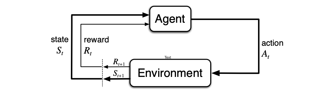
In reinforcement learning (RL), an agent takes actions in an environment to change its state over discrete timesteps $t$, with the goal of maximising the future sum of a scalar quantity known as reward. We formalise this interaction as an agent-environment loop, mathematically described as a Markov Decision Process (MDP).
MDPs break the I.I.D. data assumption of supervised and unsupervised learning; the agent causally influences the data it sees through its choice of actions. However, one assumption we do make is the Markov property, which says that the state representation captures all relevent information from the past. Formally, state transitions depend only on the most recent state and action, $$ \mathbb{P}[S_{t+1} | S_1,A_1 \ldots, S_t,A_t]=\mathbb{P}[S_{t+1} | S_t,A_t], $$ and rewards depend only on the most recent transition, $$ \mathbb{P}[R_{t+1} | S_1,A_1 \ldots, S_t,A_t,S_{t+1}] = \mathbb{P}[R_{t+1} | S_t,A_t,S_{t+1}]. $$
- Note: different sources use different notation here, but this is the most general.
In some MDPs, a subset of states are designated as terminal (or absorbing). The agent-environment interaction loop ceases once a terminal state is reached, and restarts again at $t=0$ by sampling an state from an initialisation distribution $S_0\sim\mathbb{P}_\text{init}$. Such MDPs are known as episodic, while those without terminal states are known as continuing.
The goal of an RL agent is to pick actions that maximise the discounted cumulative sum of future rewards, also known as the return $G_t$: $$ G_t = R_{t+1} + \gamma R_{t+2} + \gamma^2 R_{t+3} + \ldots + \gamma^{T-t-1}R_{T}, $$ where $\gamma\in[0,1]$ is a discount factor and $T$ is the time of termination ($\infty$ in continuing MDPs).
To do so, it needs the ability to forecast the reward-getting effect of taking each action $A$ in each state $S$, potentially many timesteps into the future. This temporal credit assignment problem is one of the key factors that makes RL so challenging.
Before we go on, it’s worth reflecting on how general the MDP formulation is. An extremely large class of problems can be cast as MDPs (it’s even possible to represent supervised learning as a special case), and this recent DeepMind paper goes as far as to say that all aspects of general intelligence can be understood as serving the maximisation of future reward. Although not everybody agrees, this attitude motivates the heavy RL focus at organisations like DeepMind and OpenAI.
1.2 MDP Example
Here’s a simple MDP (courtesy of David Silver @ DeepMind/UCL), which we’ll be using throughout this course.
- White circle: non-terminal state
- White square: terminal state
- Black circle: action
- Green: reward (depends only on $S_{t+1}$ here)
- Blue: state transition probability
- Red: action probability for an exemplar policy
- Note: edges with probability $1$ are unlabelled

1.3 Open AI Gym
Open AI Gym provides a unified framework for testing and comparing RL algorithms in Python, and offers a suite of MDPs that researchers can use to benchmark their work. It’s important to be familiar with the conventions of Gym, because almost all modern RL code is built to work with it. Gym environment classes have two key methods:
mdp.reset(): reset the MDP to an initial state $S_0$ according to the initialisation distribution $\mathbb{P}_\text{init}$.mdp.step(action): given an action $A_t$, combine with the current state $S_t$ to produce the next state according to $\mathbb{P}[S_{t+1} | S_t,A_t]$ and a scalar reward according to $\mathbb{P}[R_{t+1} | S_t,A_t,S_{t+1}]$.
A Gym-compatible class for the student MDP shown above can be found in mdp.py in this repository. Let’s import it now and explore what it can do!
from mdp import StudentMDP
mdp = StudentMDP()
Firstly, we’ll have a look at the initialisation probabilities and the behaviour of mdp.reset().
print(mdp.initial_probs())
mdp.reset()
print(mdp.state)
{'Class 1': 1.0, 'Class 2': 0.0, 'Class 3': 0.0, 'Facebook': 0.0, 'Pub': 0.0, 'Pass': 0.0, 'Asleep': 0.0}
Class 1
Next, let’s check which actions are available in this initial state, and the action-dependent transition probabilities $\mathbb{P}[S_{t+1}|\text{Class 1},A_t]$.
- Reminder: the Markov property dictates that transition probabilities depend only on the current state and action.
print(mdp.action_space(mdp.state))
print(mdp.transition_probs(mdp.state, "Study"))
print(mdp.transition_probs(mdp.state, "Go on Facebook"))
{'Study', 'Go on Facebook'}
{'Class 2': 1.0}
{'Facebook': 1.0}
Calling mdp.step(action) samples and returns the next state $S_{t+1}$, alongside the reward $R_{t+1}$. Let’s try calling this method repeatedly. What’s happening here?
state, reward, _, _ = mdp.step("Study")
print(state, reward)
Class 2 -2.0
mdp.action_space("Pass")
{'Fall asleep'}
So far, we’ve only seen deterministic transitions, but having a pint in the pub has a stochastic effect; the state goes to one of the three classes with specified probabilities.
print(mdp.action_space("Pub"))
print(mdp.transition_probs("Pub", "Have a pint"))
{'Have a pint'}
{'Class 1': 0.2, 'Class 2': 0.4, 'Class 3': 0.4}
In this state, the behaviour of mdp.step(action) changes between repeated calls, even for a constant action.
mdp.state = "Pub" # Note that we're resetting the state to Pub each time
state, reward, _, _ = mdp.step("Have a pint")
print(state, reward)
Class 2 -2.0
This MDP has just one terminal state.
print(mdp.terminal_states())
{'Asleep'}
mdp.step(action) also returns a binary done flag, which is set to True if $S_{t+1}$ is a terminal state.
mdp.state = "Class 2"
state, reward, done, _ = mdp.step("Fall asleep")
print(state, reward, done)

mdp.state = "Pass"
state, reward, done, _ = mdp.step("Fall asleep")
print(state, reward, done)
Asleep 0.0 True
Asleep 0.0 True
Now let’s bring an agent into the mix, and give it the exemplar policy shown in the diagram above.
from agent import Agent
agent = Agent(mdp)
agent.policy = {
    "Class 1":  {"Study": 0.5, "Go on Facebook": 0.5},
    "Class 2":  {"Study": 0.8, "Fall asleep": 0.2},
    "Class 3":  {"Study": 0.6, "Go to the pub": 0.4},
    "Facebook": {"Keep scrolling": 0.9, "Close Facebook": 0.1},
    "Pub":      {"Have a pint": 1.},
    "Pass":     {"Fall asleep": 1.},
    "Asleep":   {"Stay asleep": 1.}}
We can query the policy in a similar way to the MDP’s properties, and observe its stochastic behaviour.
print(agent.policy["Class 1"])
print([agent.act("Class 1") for _ in range(20)])
{'Study': 0.5, 'Go on Facebook': 0.5}
['Go on Facebook', 'Study', 'Go on Facebook', 'Study', 'Go on Facebook', 'Study', 'Go on Facebook', 'Study', 'Go on Facebook', 'Study', 'Study', 'Study', 'Go on Facebook', 'Study', 'Study', 'Study', 'Go on Facebook', 'Go on Facebook', 'Go on Facebook', 'Study']
Bringing it all together:
mdp.verbose = True
state = mdp.reset()
done = False
while not done:
    state, reward, done, info = mdp.step(agent.act(state))
=========================== EPISODE   2 ===========================
| Time  | State    | Action         | Reward | Next state | Done  |
|-------|----------|----------------|--------|------------|-------|
| 0     | Class 1  | Study          | -2.0   | Class 2    | False |
| 1     | Class 2  | Study          | -2.0   | Class 3    | False |
| 2     | Class 3  | Study          | 10.0   | Pass       | False |
| 3     | Pass     | Fall asleep    |  0.0   | Asleep     | True  |
How “good” is this policy? To answer this, we need to calculate its expected return.
2 | Policy Evaluation: The Temporal Difference Method
For a policy $\pi$, the Q value $Q_\pi(S_t,A_t)$ is the expected return from taking action $A_t$ in state $S_t$, and following $\pi$ thereafter. It thus quantifies how well the policy can be expected to perform, starting from this state-action pair. Q values exhibit an elegant recursive relationship known as the Bellman equation: $$ Q_\pi(S_t,A_t)=\sum_{S_{t+1}}\mathbb{P}[S_{t+1}|S_t,A_t]\left(\mathbb{E}[R_{t+1} | S_t,A_t,S_{t+1}]+\gamma\times\sum_{A_{t+1}}\pi(A_{t+1}|S_{t+1})\times Q_\pi(S_{t+1},A_{t+1})\right). $$
i.e. The Q value for a state-action pair is equal to the immediate reward, plus the $\gamma$-discounted Q value for the next state-action pair, with expectations taken over both the transition function $\mathbb{P}$ and the policy $\pi$.
This is a bit of a mouthful, but the Bellman equation is perhaps the single most important thing to understand if you really want to “get” reinforcement learning.
To gain some intuition for this relationship, here are estimated Q values for the exemplar policy in the student MDP. Here we’re using a discount factor of $\gamma=0.95$
- Note that these values are only approximate, so the Bellman equation doesn’t hold exactly!

To take one example: $$ Q(\text{Class 2},\text{Study})=-2+0.95\times [(0.6\times Q(\text{Class 3},\text{Study})+0.4\times Q(\text{Class 3},\text{Go to the pub}))] $$ $$ =-2+0.95\times[(0.6\times 9.99+0.4\times 1.81)] $$ $$ =4.38\approx 4.36 $$
How did we arrive at these Q value estimates? Here’s where the real magic happens.
The Bellman backup algorithm makes use of this recursive relationship to update the Q value for a state-action pair based on the current estimate of the value for the next state.
GAMMA = 0.95  # Discount factor
ALPHA = 0.001 # Learning rate

def bellman_backup(agent, state, action, reward, next_state, done):

    Q_next = 0. if done else agent.Q[next_state][agent.act(next_state)]

    agent.Q[state][action] += ALPHA * ( reward + GAMMA * Q_next - agent.Q[state][action])
By sampling episodes in our MDP using the current policy we can collect rewards and update our Q-function accordingly. The algorithm we use to evaluate policies is called policy evaluation, and it uses the Bellman back-up which has two hyperparameters $\gamma$ and $\alpha$. $\gamma$ is the discount factor that
Import the MDP and define the policy again.
from mdp import StudentMDP
from agent import Agent
mdp = StudentMDP(verbose=True)
agent = Agent(mdp)
agent.policy = {
    "Class 1":  {"Study": 0.5, "Go on Facebook": 0.5},
    "Class 2":  {"Study": 0.8, "Fall asleep": 0.2},
    "Class 3":  {"Study": 0.6, "Go to the pub": 0.4},
    "Facebook": {"Keep scrolling": 0.9, "Close Facebook": 0.1},
    "Pub":      {"Have a pint": 1.},
    "Pass":     {"Fall asleep": 1.},
    "Asleep":   {"Stay asleep": 1.}
}
Initially, we set all Q values to zero (this is actually arbitrary).
agent.Q
{'Class 1': {'Study': 0.0, 'Go on Facebook': 0.0},
 'Class 2': {'Study': 0.0, 'Fall asleep': 0.0},
 'Class 3': {'Study': 0.0, 'Go to the pub': 0.0},
 'Facebook': {'Keep scrolling': 0.0, 'Close Facebook': 0.0},
 'Pub': {'Have a pint': 0.0},
 'Pass': {'Fall asleep': 0.0},
 'Asleep': {}}
Run a single episode to see what happens.
state = mdp.reset()
done = False
while not done:
    action = agent.act(state)
    next_state, reward, done, _ = mdp.step(action)

    print('Current action value:', agent.Q[state][action])
    print('Reward obtained:', reward)
    print('Next action value:', 0. if done else agent.Q[next_state][agent.act(next_state)])

    bellman_backup(agent, state, action, reward, next_state, done)

    print('Updated action value:', agent.Q[state][action])
    print('\n')

    state = next_state
=========================== EPISODE  51 ===========================
| Time  | State    | Action         | Reward | Next state | Done  |
|-------|----------|----------------|--------|------------|-------|
| 0     | Class 1  | Study          | -2.0   | Class 2    | False |
Current action value: 4.271800760689531
Reward obtained: -2.0
Next action value: 6.9926093317691915
Updated action value: 4.272171938794022


| 1     | Class 2  | Study          | -2.0   | Class 3    | False |
Current action value: 6.9926093317691915
Reward obtained: -2.0
Next action value: 9.999149294082697
Updated action value: 6.9931159142668005


| 2     | Class 3  | Study          | 10.0   | Pass       | False |
Current action value: 9.999149294082697
Reward obtained: 10.0
Next action value: 0.0
Updated action value: 9.999150144788615


| 3     | Pass     | Fall asleep    |  0.0   | Asleep     | True  |
Current action value: 0.0
Reward obtained: 0.0
Next action value: 0.0
Updated action value: 0.0
Repeating a bunch of times, we gradually converge.
mdp.verbose = False

print('Initial Q')
print(agent.Q)

for _ in range(20000):
    state = mdp.reset()
    done = False
    while not done:
        action = agent.act(state)
        next_state, reward, done, _ = mdp.step(action)
        bellman_backup(agent, state, action, reward, next_state, done)
        state = next_state

print('\n')
print('Converged Q')
print(agent.Q)
Initial Q
{'Class 1': {'Study': -0.002, 'Go on Facebook': -0.001}, 'Class 2': {'Study': -0.002, 'Fall asleep': 0.0}, 'Class 3': {'Study': 0.01, 'Go to the pub': 0.0}, 'Facebook': {'Keep scrolling': -0.0049995000249993754, 'Close Facebook': -0.00200095}, 'Pub': {'Have a pint': 0.0}, 'Pass': {'Fall asleep': 0.0}, 'Asleep': {}}


Converged Q
{'Class 1': {'Study': 1.3750628761712569, 'Go on Facebook': -11.288976651525505}, 'Class 2': {'Study': 4.485658109648779, 'Fall asleep': 0.0}, 'Class 3': {'Study': 9.999996524778595, 'Go to the pub': 1.8953439336946862}, 'Facebook': {'Keep scrolling': -11.233042781986304, 'Close Facebook': -6.6761905244797735}, 'Pub': {'Have a pint': 0.9312667143217461}, 'Pass': {'Fall asleep': 0.0}, 'Asleep': {}}
Note that although the policy evaluation process is guaranteed to converge eventually (for simple MDPs!), we are likely to see some discrepencies between runs of finite length because of the role of randomness in the data collection process. Here are the results of five independent repeats:
{'Class 1': {'Study': 1.2650695038546025, 'Go on Facebook': -11.30468184426212}, 'Class 2': {'Study': 4.407552596737938, 'Fall asleep': 0.0}, 'Class 3': {'Study': 9.99999695776742, 'Go to the pub': 1.8487809354712246}, 'Facebook': {'Keep scrolling': -11.258053618560483, 'Close Facebook': -6.489974573408375}, 'Pub': {'Have a pint': 0.9454014270087486}, 'Pass': {'Fall asleep': 0.0}, 'Asleep': {}}
{'Class 1': {'Study': 1.3338704627380917, 'Go on Facebook': -11.222578014516461}, 'Class 2': {'Study': 4.404498313710967, 'Fall asleep': 0.0}, 'Class 3': {'Study': 9.999996607231745, 'Go to the pub': 1.9330819535637127}, 'Facebook': {'Keep scrolling': -11.237574593720579, 'Close Facebook': -6.649035509952115}, 'Pub': {'Have a pint': 1.0198591832482675}, 'Pass': {'Fall asleep': 0.0}, 'Asleep': {}}
{'Class 1': {'Study': 1.255108027766012, 'Go on Facebook': -11.190843458457234}, 'Class 2': {'Study': 4.3028079916966, 'Fall asleep': 0.0}, 'Class 3': {'Study': 9.999996368375, 'Go to the pub': 1.692402249138645}, 'Facebook': {'Keep scrolling': -11.009224020468848, 'Close Facebook': -6.456279660637165}, 'Pub': {'Have a pint': 0.7467114530860179}, 'Pass': {'Fall asleep': 0.0}, 'Asleep': {}}
{'Class 1': {'Study': 1.2734946938741027, 'Go on Facebook': -11.328006914127434}, 'Class 2': {'Study': 4.256107269897298, 'Fall asleep': 0.0}, 'Class 3': {'Study': 9.99999635381211, 'Go to the pub': 1.74113336614775}, 'Facebook': {'Keep scrolling': -11.34039736455563, 'Close Facebook': -6.777709970724558}, 'Pub': {'Have a pint': 0.7694312629253455}, 'Pass': {'Fall asleep': 0.0}, 'Asleep': {}}
{'Class 1': {'Study': 1.2650695038546025, 'Go on Facebook': -11.30468184426212}, 'Class 2': {'Study': 4.407552596737938, 'Fall asleep': 0.0}, 'Class 3': {'Study': 9.99999695776742, 'Go to the pub': 1.8487809354712246}, 'Facebook': {'Keep scrolling': -11.258053618560483, 'Close Facebook': -6.489974573408375}, 'Pub': {'Have a pint': 0.9454014270087486}, 'Pass': {'Fall asleep': 0.0}, 'Asleep': {}}
{'Class 1': {'Study': 1.2650695038546025,
  'Go on Facebook': -11.30468184426212},
 'Class 2': {'Study': 4.407552596737938, 'Fall asleep': 0.0},
 'Class 3': {'Study': 9.99999695776742, 'Go to the pub': 1.8487809354712246},
 'Facebook': {'Keep scrolling': -11.258053618560483,
  'Close Facebook': -6.489974573408375},
 'Pub': {'Have a pint': 0.9454014270087486},
 'Pass': {'Fall asleep': 0.0},
 'Asleep': {}}
Try with $\gamma=0$
3 | Policy Improvement

Having evaluated our policy $\pi$, how can we go about obtaining a better one? This question is the heart of policy improvement, perhaps the fundamental concept of RL. Recall, when we performed policy evaluation we obtained the value of taking every action in every state. Thus, we can perform policy improvement readily by picking our current best estimate of the optimal action from each state – so-called greedy action selection. Once we’ve obtained a new policy, we can evaluate it as before. Continually iterating between policy evaluation and policy improvement in this way, we are guarenteed to reach the optimal policy $\pi^*$ according to the policy improvement theorem.
3.1 | Q-learning: Combining Policy Evaluation and Improvement

from mdp import StudentMDP
mdp = StudentMDP(verbose=True)
from agent import QLearningAgent
agent = QLearningAgent(mdp, epsilon=1.0, alpha=0.2, gamma=0.9)
NUM_EPS = 50
mdp.ep = 0
while mdp.ep < NUM_EPS:
    state = mdp.reset()
    done = False
    while not done:
        action = agent.act(state)
        next_state, reward, done, info = mdp.step(action)
        agent.learn(state, action, reward, next_state, done)
        state = next_state

    print("Value function:")
    print(agent.Q)
    print("Policy:")
    print(agent.policy)
    print("Epsilon:", agent.epsilon)

    agent.epsilon = max(agent.epsilon - 1 / (NUM_EPS-1), 0)
=========================== EPISODE   1 ===========================
| Time  | State    | Action         | Reward | Next state | Done  |
|-------|----------|----------------|--------|------------|-------|
| 0     | Class 1  | Study          | -2.0   | Class 2    | False |
| 1     | Class 2  | Study          | -2.0   | Class 3    | False |
| 2     | Class 3  | Study          | 10.0   | Pass       | False |
| 3     | Pass     | Fall asleep    |  0.0   | Asleep     | True  |
Value function:
{'Class 1': {'Study': -0.4, 'Go on Facebook': 0.0}, 'Class 2': {'Study': -0.4, 'Fall asleep': 0.0}, 'Class 3': {'Study': 2.0, 'Go to the pub': 0.0}, 'Facebook': {'Keep scrolling': 0.0, 'Close Facebook': 0.0}, 'Pub': {'Have a pint': 0.0}, 'Pass': {'Fall asleep': 0.0}, 'Asleep': {}}
Policy:
{'Class 1': {'Study': 0.5, 'Go on Facebook': 0.5}, 'Class 2': {'Study': 0.5, 'Fall asleep': 0.5}, 'Class 3': {'Study': 0.5, 'Go to the pub': 0.5}, 'Facebook': {'Keep scrolling': 0.5, 'Close Facebook': 0.5}, 'Pub': {'Have a pint': 1.0}, 'Pass': {'Fall asleep': 1.0}, 'Asleep': {}}
Epsilon: 1.0

=========================== EPISODE  50 ===========================
| Time  | State    | Action         | Reward | Next state | Done  |
|-------|----------|----------------|--------|------------|-------|
| 0     | Class 1  | Study          | -2.0   | Class 2    | False |
| 1     | Class 2  | Study          | -2.0   | Class 3    | False |
| 2     | Class 3  | Study          | 10.0   | Pass       | False |
| 3     | Pass     | Fall asleep    |  0.0   | Asleep     | True  |
Value function:
{'Class 1': {'Study': 4.2185955736170015, 'Go on Facebook': -2.843986498540236}, 'Class 2': {'Study': 6.978887265282676, 'Fall asleep': 0.0}, 'Class 3': {'Study': 9.997403851570732, 'Go to the pub': 1.0297507967148403}, 'Facebook': {'Keep scrolling': -3.2301556459908016, 'Close Facebook': -0.8716820424598939}, 'Pub': {'Have a pint': 2.6089417712654472}, 'Pass': {'Fall asleep': 0.0}, 'Asleep': {}}
Policy:
{'Class 1': {'Study': 1.0, 'Go on Facebook': 0.0}, 'Class 2': {'Study': 1.0, 'Fall asleep': 0.0}, 'Class 3': {'Study': 1.0, 'Go to the pub': 0.0}, 'Facebook': {'Keep scrolling': 0.0, 'Close Facebook': 1.0}, 'Pub': {'Have a pint': 1.0}, 'Pass': {'Fall asleep': 1.0}, 'Asleep': {}}
Epsilon: 0
We find that after 50 episodes the agent has obtained the optimal policy $\pi_*$!
4 | Deep RL
So far, we’ve tabularised the state-action space. Whilst useful for explaining the fundamental concepts that underpin RL, the real world state-action spaces are generally continuous and thus impossible to tabularise. To combat this, function approximators are used instead. In the past these included x, but more recently, deep neural networks have been used giving rise to the field of Deep Reinforcement Learning.
The seminal Deep RL algorithm is Deep Q Learning which uses neural networks to represent the $Q$ function. The network takes the current obervation $o_t$ as input and predicts the value of each action. The agent’s policy is $\epsilon$-greedy as before i.e. it takes the value-maximising action with probability $1 - \epsilon$. Deep Q learning
Below, we run 500 episodes of the canonical Cartpole task using Deep Q learning. The agent’s goal is to balance the pole in the upright position for as long as possible starting from an initially random position.
import gym
from dqn_agent import Agent
import numpy as np
env = gym.make('CartPole-v1')
agent = Agent(gamma=0.99, epsilon=0.9, lr=0.0001, n_actions=env.action_space.n, input_dims=[env.observation_space.shape[0]],
              mem_size=50000, batch_size=128,  eps_dec=1e-3, eps_min=0.05, replace=1000,
              env_name='cartpole', chkpt_dir='tmp/dqn')

best_score = -np.inf
episodes = 500
scores, avg_score, eps_history = [], [], []

for i in range(episodes):
    score = 0
    done = False
    observation = env.reset()
    env.render()
    while not done:
        action = agent.choose_action(observation)
        observation_, reward, done, info = env.step(action)
        score += reward
        agent.store_transition(observation, action, reward, observation_, done)
        agent.learn()
        observation = observation_
        env.render()

    scores.append(score)
    eps_history.append(agent.epsilon)

    avg_score = np.mean(scores[-100:])

    print('episode', i, 'score %.2f' % score, 'average score %.2f' % avg_score)
5 | What Did We Miss Out?
- Dynamic programming (when transition probabilities are known)
- Monte Carlo
- Exploration strategies
- Continuous actions
- Policy gradient, actor-critic
- Model-based
- Partial observability
What next? RL interest group?