Reinforcement Learning for Energy Efficient Control
Cambridge Zero Symposia
17th November 2021, 3pm
Abstract
Energy use in buildings accounts for 39% of global emissions, much of which are regulated by Rule Based Controllers (RBC) that neither maximise energy efficiency nor minimise emissions by interacting optimally with the grid. In this talk, I introduce a new method for controlling buildings using probabilistic deep reinforcement learning that is capable of reducing emissions after only a few hours of deployment with no prior knowledge. I present results from experiments conducted in three varied building energy simulations, and show my approach outperforms an existing RBC twice, and the state-of-the-art RL algorithms in all cases, reducing emissions by as much as 30.00% whilst maintaining thermal comfort.
Code
![]()
Slides
Notes
My name’s Scott Jeen, I’m a second year PhD student in the department of engineering looking at Reinforcement Learning, and its applications for mitigating climate change. My talk today is titled Reinforcement Learning for Energy Efficient Control, and it’s going to provide a high-level summary of the work carried out in the first year of my PhD. I’ll start by describing and motivating the problem we are trying to solve.
1. Motivation
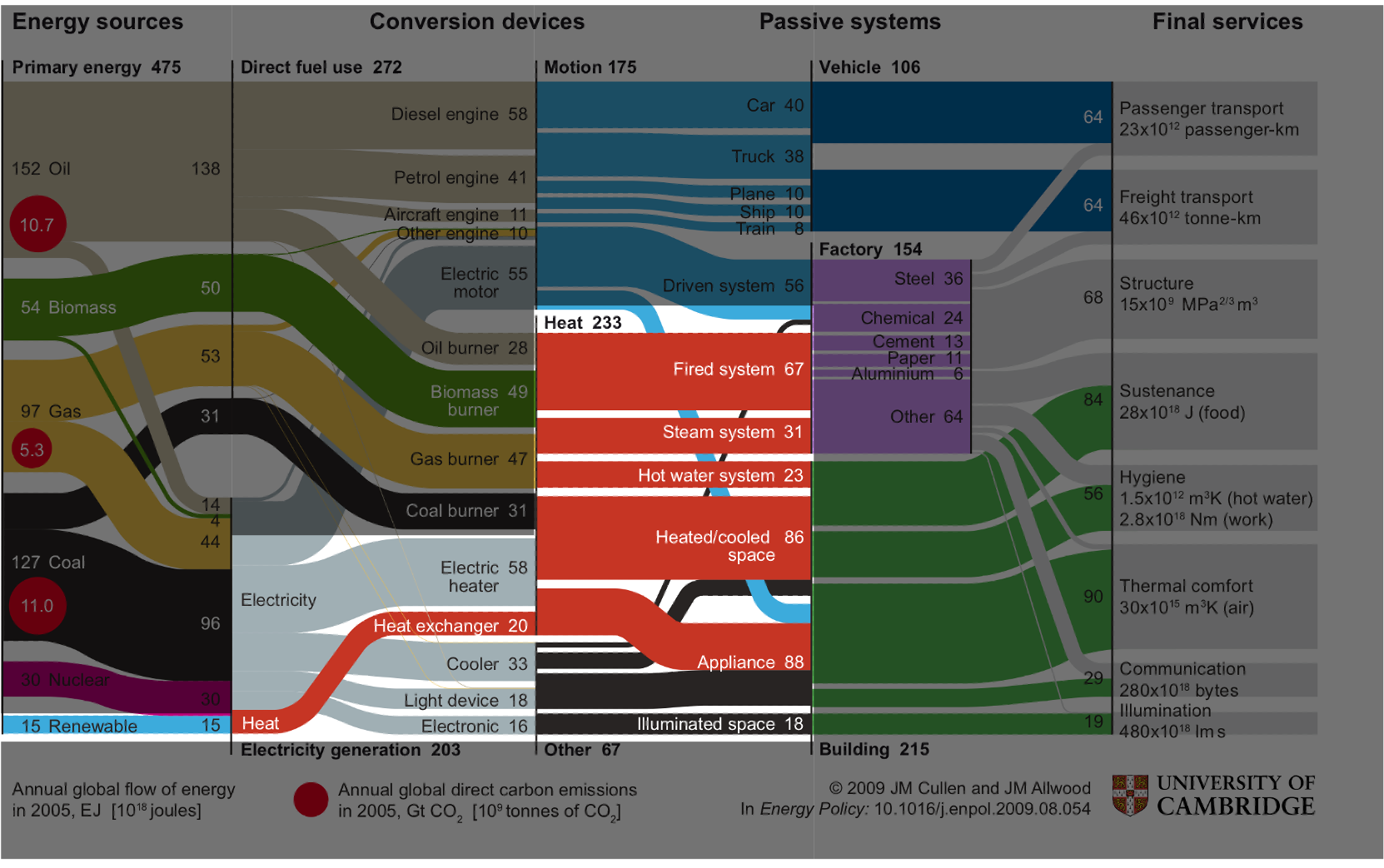
Here’s a diagram my supervisor Jon Cullen produced a few years ago mapping global energy sources, on the left hand-side of the diagram, through conversion devices, to final services on the right hand-side of the diagram. Though it looks complicated, I’d like to simplify things by focussing your attention on the middle section of the diagram.

Here we see that global energy use can be stratified into one of three categories: energy used to create motion in cyan; energy used to regulate temperature in red; and energy used for everything else in black. We can observe that the primary source of energy consumption globally is in regulating temperature - approximately 50% of total energy demand. Finding ways of regulating temperature in society more efficiently would prove a useful way of reducing energy use and this carbon emissions.

Another part of the diagram I’d like to draw your attention to is the blue sliver labelled renewables in the bottom left. Though renewables contributed to a small percentage of global energy supply when this diagram was produced (using data from 2005), the International Energy Agency expect renewables to contribute to 75% of global energy supply by 2050. Such a high penetration of renewables on the grid will cause problems, problems related primarily to the stochastic nature of renewable energy generation - often called its intermittency.
To explain intermittency, consider the hypothetical scenario of powering a home using only a solar array located on its roof. Here, we plot demand for energy in blue and the supply of energy from the solar array in orange, for 24 hours. On a perfectly clear summers day, the energy supplied by our solar array will increase in the morning as the sun rises, peak around midday when irradiance is highest, and fall in the evening as the sun sets. In contrast, the occupant’s demand for energy won’t be so symmetric. They’ll likely demand produce a peak in energy demand in the morning when they wake up, boil the kettle, turn the heating on and take a shower. Then, they’ll head out to work and demand will fall and plateau. In the evening they’ll return causing another spike in energy demand as the heating comes on, they cook dinner and turn on a range of appliances.

These mismatched curves create periods where we have surplus power supply (green) and periods where we have a deficit (red). Where demand exceeds supply, as is the case in the evening, the national grid will cover the deficit by spinning up a gas-powered power station (a process called peak-matching), doing so creates unnecessary emissions that could have been avoided if we had shifted surplus power created during the day to the evening.

Here is an illustration of such an idealised scenario. Now we’ve added a storage medium, this could be a chemical storage i.e. a battery, or it could be thermal storage i.e. thermal inertia in building materials. We’ve flattened the blue demand curve, spreading it throughout the day rather than allowing the peaks in the morning and evenings. Now we store our surplus energy during the day in orange, and discharge it in the mornings and evening in blue. In this scenario we avoid the unnecessary spinning up of the gas-powered power plant and reduce overall emissions.

Equipment in most buildings are regulated by Rule-based Controllers (RBCs) that take system temperature as input, use a temperature setpoint as an objective, and actuate equipment to minimise the error between objective and state. Though usefully simple, they don’t maximise energy efficiency, nor do they interact with the grid to draw power when carbon intensity is low to minimise emissions. We’d like to design controllers that learn patterns in occupant behaviour, weather, and grid carbon intensity and take control actions that move us toward this idealised scenario that minimises emissions. For that, in my work, I employ Reinforcement Learning (RL), a method for obtaining optimal control polices in complex systems autonomously.
2. Existing Solutions
This area has been well studied in recent years, with some authors suggesting they can achieve energy efficiency improvements of up to 30% using RL. Much of this work has employed the most popular RL paradigm: model-free reinforcement learning.
2.1 Model-free Reinforcement Learning
| Rollouts | Network |
|---|---|
 |
 |
In model free RL, our agent learns policy that is a mapping from state to action, represented by the network diagram on the right. On the left, we visualise how an RL agent collects experience in an environment to learn this mapping. The agent will start in some state $s_t$ where it takes some action $a_t$ transitioning it to some next state $s_{t+1}$, from which it takes another action $a_{t+1}$. This process continues until some finite time horizon $H$ where it will receive some reward, a quantification of how good the previous string of actions were. This reward is backpropogated, and the network is updated to reflect how good or bad each of those actions were at achieving our goal.
As may be clear, to obtain an optimal solution, the agent would have to visit all possible states and take all possible actions. To do this safely, these agents are usually obtained in building simulations using millions of timesteps of data, but such simulations can be difficult, expensive or impossible to obtain in some buildings, so this approach limits the applicability of model-free RL to the subset of global buildings for which we have can obtain such data in advance.
2.2 Model-based Reinforcement Learning
| Rollouts | Network |
|---|---|
 |
 |
An alternative is model-based RL where the agent instead learns a mapping from state-action pair to next state, in other words, it attempts to learn the system dynamics. Using this model, the agent can test a range of candidate action sequences, estimating the expected reward of each at time horizon $H$. The agent then takes the first action from the action sequence producing highest expected reward in the real world.
This approach is considerably more data-efficient than model-free RL because the agent can imagine the consequences of as many actions as it likes offline, limiting the amount of interactions required in the real environment to obtain a good policy. Because of this, authors have shown that model-based RL agents do not need to be pre-trained in simulation, but can instead be deployed directly in the environment where it can learn a policy after 12 hours of interaction. However, the primary drawback is that the model it learns is inevitably wrong to some degree, or biased, and this model inaccuracy can lead to poorer performance than model-based agents.
| Pros 💚 | Cons 💔 | |
|---|---|---|
| Model-free | Performance | Data inefficiency |
| Model-based | Data efficiency | Performance; Model bias |
| Energy Efficiency | Data Efficiency | Authors | |
|---|---|---|---|
| SOA Model-free | 10-30% | 1-2 years simulated data | [2,3] |
| SOA Model-based | 5-9% | 3-12 hours live data | [4, 5] |
Here I summarise the pros and cons of each approach. In general, model-free approaches perform better but are data inefficient - requiring pre-training in a simulator. On the other hand, model-based techniques are far more data efficient, but model-bias can cause poorer performance. We see this reflected in the building control literature, where model-free approaches have shown energy efficiency improvements of up to 30%, whereas model-based techniques have only shown up to 9% energy efficiency improvements.
Ideally, we’d like to find new solutions that elicit the performance of model-free approaches with the data efficiency and online commissioning of model-based approaches. The approach we propose for doing so is Probabilistic Model-Based Reinforcement Learning.
3. Probabilisitic Model-Based Reinforcement Learning
Here we follow the same schema as traditional model-based RL i.e. we learn a mapping from state-action pair to next state, but now instead of deterministically predicting the state evolution, we learn a probability distribution over next state parameterised by mean $\mu$ and variance $\sigma$. We employ an ensemble of 5 probabilistic networks to account for uncertainty in the modelling approach too.

after [6]
The method for agent planning changes too, now instead of making point predictions of the outcome of action sequences, we output a distribution over all possible future rewards. In the example below, we evaluate one action sequence, passing it through three models in our ensemble, outputting state distribution predictions, sampling from that distribution and iterating until time horizon $H$. At this stage we get a distribution over rewards which we can use to get the expected value of the action sequence. Comparing this with the expected reward of many other action sequences we can find the optimal action sequence, and take the first action in that sequence in the real environment.

4. Experiments
We ran a series of experiments to test the effectiveness of our proposed approach. We test our algorithm in three varied building simulations, a mixed-use facility in Greece, an apartment block in Spain, and a seminar centre in Denmark. We compare our algorithm with an existing RBC, the state-of-the-art model-free approach and the state-of-the-art model-based approach. The agents have no prior knowledge of the system a priori, other than the type of actions they can take, and are each given 12 hours to explore the state-space before controlling them. The goal of each agent is to minimise emissions whilst maintaining internal temperature in the range 19-24 degrees centigrade for one year of operation.
4.1 Building Simulations [7]


Figure 1: Building energy simulation schematics. Top: Mixed Use; Middle: Apartment; Bottom: Seminar Centre.
We find that in two of the three cases our PMBRL method (green) minimises emissions over all other controllers. In the mixed-use facility it reduces emissions by 30% over the RBC and in the apartment block it reduces emissions by 10%. In the seminar centre it creates the same volume of emissions as the existing controller.
4.2 Emissions

Figure 2: Cumulative emissions produced by each controller across the (a) Mixed Use, (b) Apartment, and (c) Seminar Centre environments. Green: PMBRL; Orange: PPO; Blue: MPC-DNN; Red: RBC.
Our approach is also the best at maintaining temperature within the desired bounds, here represented by the light green band. Our approach never breaches the temperature bounds in the apartment or seminar centre, and does so 0.27% of the year in the mixed use facility. In contrast the existing SOA approaches breach the same bounds 18.36% (model-based) and 53.33% (model-free) of the time on average.
4.3 Thermal Comfort

Figure 3: Mean daily building temperature produced by each controller across the (a) Mixed Use, (b) Apartment, and (c) Seminar Centre environments. Green: PMBRL; Orange: PPO; Blue: MPC-DNN; Red: RBC; Purple Dashed: Outdoor temperature (the primary system disturbance). The green shaded area illustrates the target temperature range [19, 24].
5. Conclusions
- Reducing energy use in heating and cooling systems, and better matching energy demand with carbon-free supply are important climate change mitigation tools.
- In theory, RL allows us to obtain emission-reducing control policies for any building with no prior knowledge.
- Existing RL approaches require training in hard-to-obtain simulators using millions of timesteps of data.
- Our approach, PMBRL, is easy to deploy, requiring no prior knowledge, and can obtain emission-reducing control policies after only a few hours of interaction in the real environment.
Thanks!

Twitter: @enjeeneer
Website: https://enjeeneer.io/
6. References
[1] Cullen, Jonathan and Julian Allwood (2010). “The efficient use of energy: Tracing the global flow of energy from fuel to service”. In: Energy Policy 38.1, pp. 75–81.
[2] Zhang, Z., Chong, A., Pan, Y., Zhang, C., Lam, K.P.: Whole building energy model for hvac optimalcontrol: A practical framework based on deep reinforcement learning. Energy and Buildings199,472–490 (2019)
[3] Wei, T., Wang, Y., Zhu, Q.: Deep reinforcement learning for building hvac control. In: Proceedingsof the 54th Annual Design Automation Conference 2017. DAC ’17, Association for ComputingMachinery, New York, NY, USA (2017).
[4] Lazic, N., Lu, T., Boutilier, C., Ryu, M., Wong, E.J., Roy, B., Imwalle, G.: Data center cooling usingmodel-predictive control. In: Proceedings of the Thirty-second Conference on Neural InformationProcessing Systems (NeurIPS-18). pp. 3818–3827. Montreal, QC (2018)
[5] Jain, A., Smarra, F., Reticcioli, E., D’Innocenzo, A., Morari, M.: Neuropt: Neural network basedoptimization for building energy management and climate control. In: Bayen, A.M., Jadbabaie, A.,Pappas, G., Parrilo, P.A., Recht, B., Tomlin, C., Zeilinger, M. (eds.) Proceedings of the 2nd Confer-ence on Learning for Dynamics and Control. Proceedings of Machine Learning Research, vol. 120,pp. 445–454
[6] Chua, K., Calandra, R., McAllister, R., Levine, S.: Deep reinforcement learning in a handful oftrials using probabilistic dynamics models. arXiv preprint arXiv:1805.12114 (2018)
[7] Scharnhorst, P., Schubnel, B., Fern ́andez Bandera, C., Salom, J., Taddeo, P., Boegli, M., Gorecki, T.,Stauffer, Y., Peppas, A., Politi, C.: Energym: A building model library for controller benchmarking.Applied Sciences11(8), 3518 (2021)