Zero Shot Building Control
OXCAV, Dept. of Computer Science, University of Oxford
Abstract
Heating and cooling systems in buildings account for 31% of global energy use, much of which are regulated by Rule Based Controllers (RBCs) that neither maximise energy efficiency nor minimise emissions by interacting optimally with the grid. Control via Reinforcement Learning (RL) has been shown to significantly improve building energy efficiency, but existing solutions require pre-training in simulators that are prohibitively expensive to obtain for every building in the world. In response, we show it is possible to perform safe, zero-shot control of buildings by combining ideas from system identification and model-based RL. We call this combination PEARL (Probabilistic Emission-Abating Reinforcement Learning) and show it reduces emissions without pre-training, needing only a three hour commissioning period. In experiments across three varied building energy simulations, we show PEARL outperforms an existing RBC once, and popular RL baselines in all cases, reducing building emissions by as much as 31% whilst maintaining thermal comfort.
Code
![]()
Slides
Outline
- Motivation: Climate Change Mitigation, Intermittency, and Smart Building Control
- Existing Work
- PEARL: Probabilistic Emission-Abating Reinforcement Learning
- Experimental Setup
- Results and Discussion
- Limitations, Future Work and Conclusions
1. Motivation: Climate Change Mitigation, Intermittency, and Smart Building Control
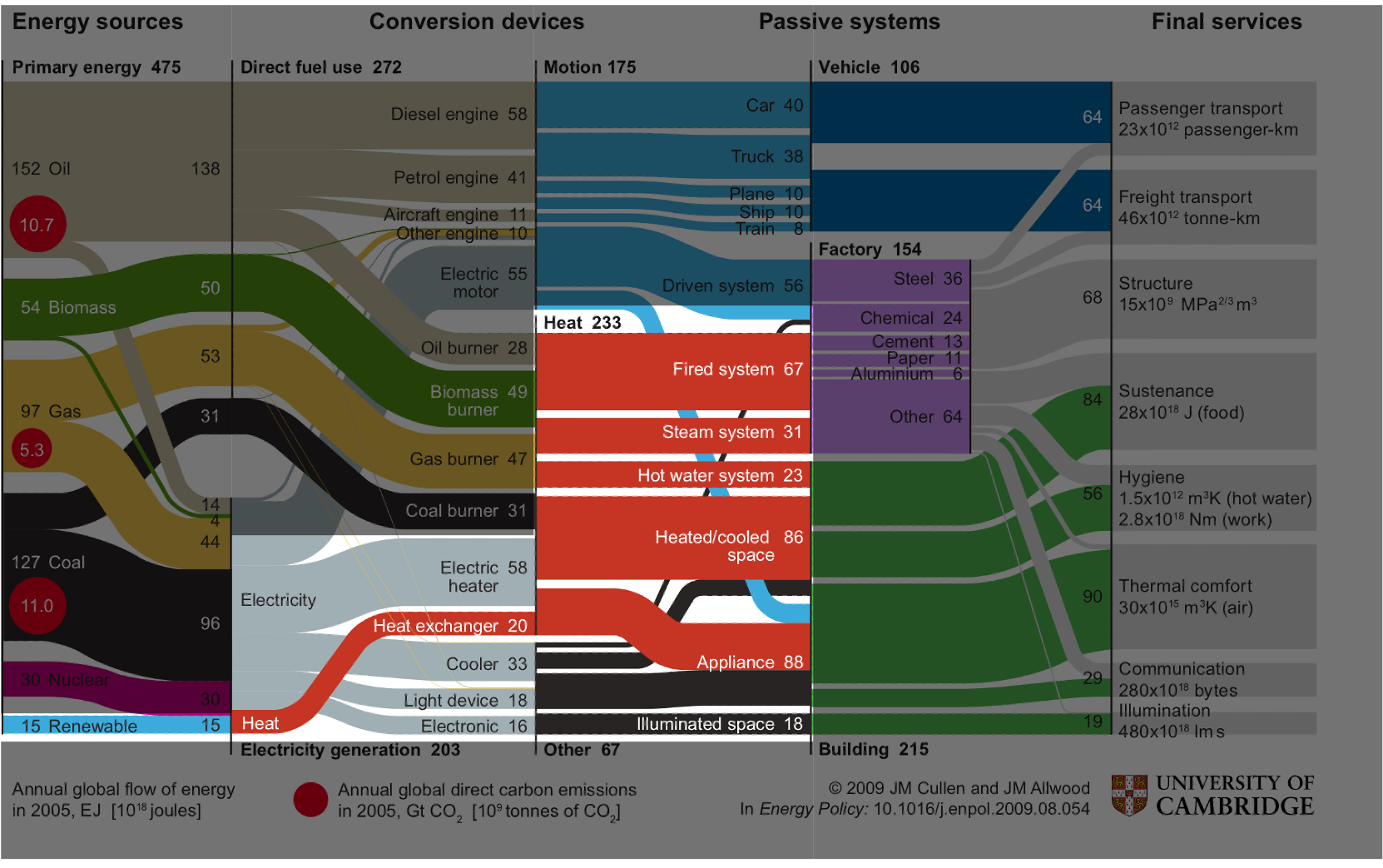
Here’s a diagram my supervisor Jon Cullen produced a few years ago mapping global energy sources, on the left handside of the diagram, through conversion devices, to final services on the right handside of the diagram. Though it looks complicated, I’d like to simplify things by focussing your attention on the middle section of the diagram.

Cullen and Allwood (2010)
Here we see that global energy use can be stratified into one of three categories: energy used to create motion in cyan; energy used to regulate temperature in red; and energy used for everthing else in black. We can observe that the primary source of energy consumption globally is in regulating temperature - approximately 50% of total energy demand. Finding ways of regulating temperature in society more efficiently would prove a useful way of reducing energy use and thus carbon emissions.

Another part of the diagram I’d like to draw your attention to is the blue sliver labelled renewables in the bottom left. Though renewables contributed to a small percentage of global energy supply when this diagram was produced (using data from 2005), the International Energy Agency expect renewables to contribute to 75% of global energy supply by 2050. Such a high penetration of renewables on the grid will cause problems, problems related primarily to the stochastic nature of renewable energy generation - often called its intermittency.
To explain intermittency, consider the hypothetical scenario of powering a home using only a solar array located on its roof. Here, we plot demand for energy in blue and the supply of energy from the solar array in orange, for 24 hours. On a perfectly clear summers day, the energy supplied by our solar array will increase in the morning as the sun rises, peak around midday when irradiance is highest, and fall in the evening as the sun sets. In contrast, the occupant’s demand for energy won’t be so symmetric. They’ll likely produce a peak in energy demand in the morning when they wake up, boil the kettle, turn the heating on and take a shower. Then, they’ll head out to work and demand will fall and plateau. In the evening they’ll return causing another spike in energy demand as the heating comes on, they cook dinner and turn on a range of appliances.
1.2 Intermittency

These mismatched curves create periods where we have surplus power supply (green) and periods where we have a deficit (red). Where demand exceeds supply, as is the case in the evening, the national grid will cover the deficit by spinning up a gas-powered power station (a process called peak-matching), doing so creates unneccesary emissions that could have been avoided if we had shifted surplus power created during the day to the evening.
1.2 Intermittency
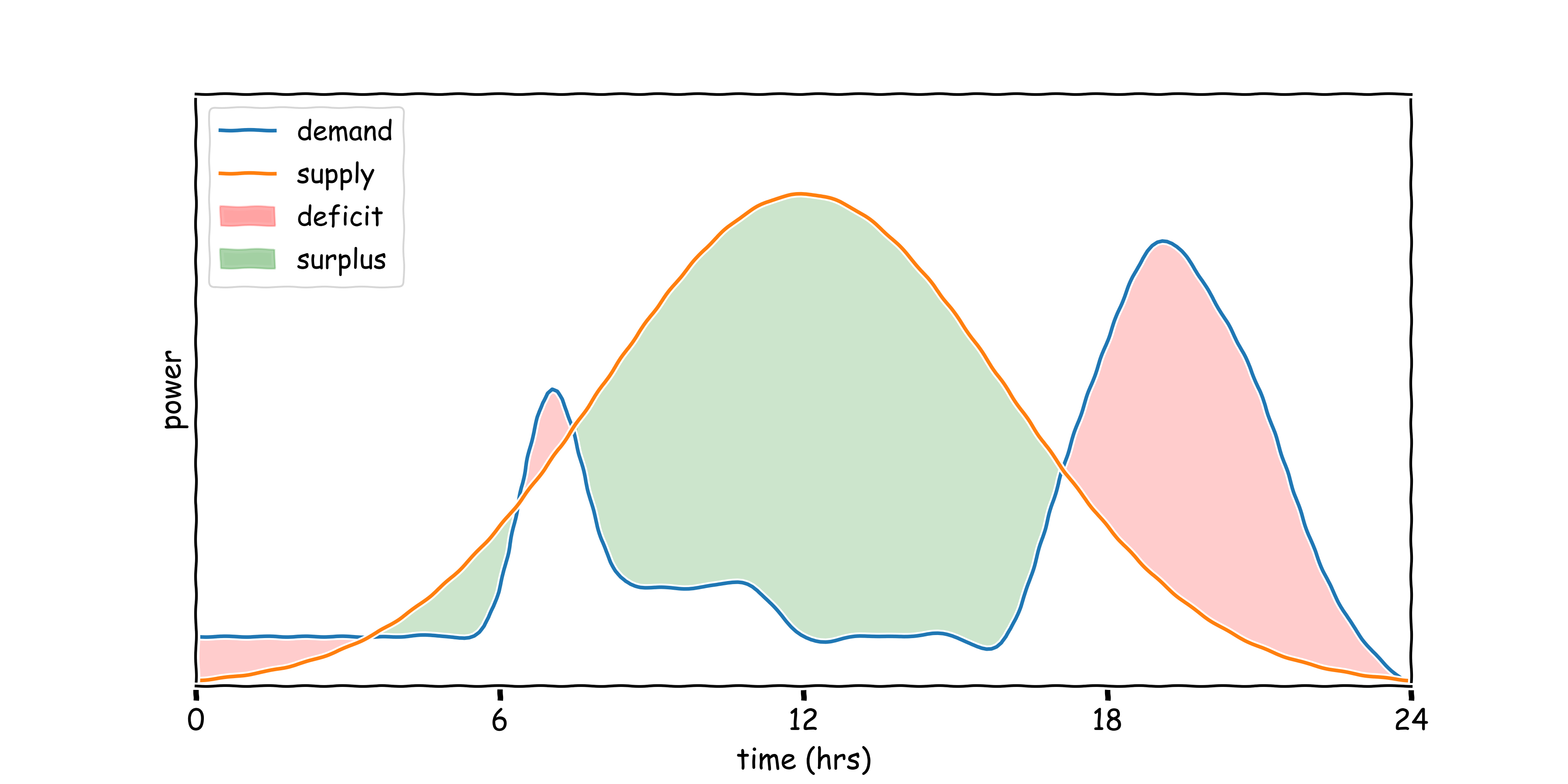
Here is an illustration of such an idealised scenario. Now we’ve added a storage medium, this could be a chemical storage i.e. a battery, or it could be thermal storage i.e. thermal inertia in building materials. We’ve flattened the blue demand curve, spreading it throughout the day rather than allowing the peaks in the morning and evenings. Now we store our surplus energy during the day in orange, and discharge it in the mornings and evening in blue. In this scenario we avoid the unnecessary spinning up of the gas-powered power plant and reduce overall emissions.
Clearly, traditional controllers cannot perform this optimisation, so we need new techniques to do so; I’m interested in Reinforcement Learning as a solution, with it’s strength being an ability to obtain polices tabula rasa, and updating system understanding online as the environment evolves.
1.3 Smart Building Control

2. Existing Work
Let’s have a look at the existing work applying RL to the task of smart building control. Most existing work has applied model-free RL algorithms, three of which are listed in the table. The general schema is as follows:
- simulate the dynamics of a real building in a physics-simulator like EnergyPlus;
- train agent for millions of timesteps in said simulation until policy converges;
- deploy agent in real building and hope simulator was sufficiently accurate that the policy transfers;
- observe energy efficiency improvement up to 35%.
The fundamental problem with this approach is that the simulators required for pre-training are both necessary and expensive to obtain, often taking experts months to produce whilst requiring significant prior knowledge.
2.1: Model-free RL for Smart Building Control

| Authors | Setting | Algorithm | Energy Efficiency | Data Efficiency | In-Situ |
|---|---|---|---|---|---|
| Wei et al. (2017) | 5-zone Building | Deep Q-Learning | ~35% | ~8 years in simulation | ❌ |
| Zhang et al. (2019a) | Office | A3C | ~17% | ~30 years in simulation | ✅ |
| Valladares et al. (2019) | Classroom | Double Q Learning | 5% | ~10 years in simulation | ✅ |
An alternative, as proposed by Lazic et al. (2018), is to grant agents a short commissioning period of 3-12 hours in the real environment. Doing so is suitably general for scaled deployment, but their agent only improved cooling costs by 9% in experiments conducted for one day, poorer performance than the agents trained in simulation. Eliciting the performance of model-free agents trained in simulation whilst training on limited data from real environments remains an open problem.
2.2: Model-based RL for Smart Building Control

| Authors | Setting | Algorithm | Energy Efficiency | Data Efficiency | In-Situ |
|---|---|---|---|---|---|
| Lazic et al. (2018) | Datacentre | MPC with Linear Model | ~9% | 3 hours live data | ✅ |
So this work is based on the critical assumption that scaling agent deployment to every building in the world necessitates bypassing expensive-to-obtain simulators and performing zero-shot control. Our goal is to find new that are as data-efficient as Lazic et al. (2018) (i.e ~ 3 hours of live data), yet perform as well as Wei et al. (2017) (i.e. ~ 35% reduction in energy).
2.3: This Work
Assumption
To scale to every building in the world, we must bypass expensive-to-obtain simulators and perform zero-shot control.
Goal
Find new methods that are as data-efficient as Lazic et al. (2018) (i.e ~ 3 hours of live data), yet perform as well as Wei et al. (2017) (i.e. ~ 35% reduction in energy)
3. PEARL: Probabilistic Emission-Abating Reinforcement Learning
I’ll now talk you through the method we propose for performing zero-shot control of buildings which we call PEARL: Probabilistic Emission-Abating Reinforcement Learning. I want to make clear that none of the components are themselves novel, but they are yet to be arranged in the way I’ll propose. I also want to make clear that the core contribution of this paper is not this approach, this is just the approach we use to show that zero-shot control is indeed possible, and we needed this because existing approaches to smart building are not adequate for the task.
3.1 End-to-end Agent

System ID: Lazic et al. (2018)
Probabilistic Ensembles: Lakshminarayanan et al. (2017)
Trajectory Sampling, CEM and MPC: Botev et al. (2013) and Chua et al. (2018)
Pearl has four components: 1) a system identification policy that follows the work of Lazic et al. (2018), that feeds into 2) a probabilistic ensemble of deep networks that follows the work of Lakshminarayanan et al. (2017). Planning is performed using Trajectory Sampling, as proposed by Chua et al. (2018), and actions are selected by optimising with Cross-Entropy Maximisation (Botev et al. (2013)) and Model Predictive Control.
I’ll take each of these components to provide more detail.
3.2 System Identification
During a Commissioning Period, \( \pi_{systemID} \) is a uniform random walk in control space, bounded to a safe range, with bounded stepwise changes:
$$ a^i[t+1] = \max\left(a_{min}^i, \min(a_{max}^i, a^i[t] + v^i)\right), v^i \sim \text{Uniform}\left(- \Delta ^i, \Delta^i\right) ; ; ; ; ; (1) $$
where:
\(a^i[t]\) is the value of action \(i\) at timestep \(t\), with \(i \in \mathcal{A}\);
[\(a_{min}^i\), \(a_{max}^i\)] is the safe operating range for action \(i\); and
\(\Delta^i\) is the maximum allowable change in action \(a^i\) between timesteps.
First, the system identification policy. During a commissioning period, the agent performs a uniform random walk in control space, bounded to a safe range with bounded stepwise changes (equation 1). All we’re saying in Equation 1 is that a proposed change the action is sampled from a uniform distribution of safe hardware changes, and we add that delta to the previous action as long as its not above or below the maximum and minimum operating range informed by historical data.
3.3 Learned Dynamics
Approximate one-step dynamics: \(\tilde{f_{\theta}}: (s_t, a_t) \rightarrow s_{t+1}\)
Output: \(\tilde{f_\theta}(s_t, a_t) = \mathcal{N}(\mu_\theta(s_t, a_t), \Sigma_\theta(s_t, a_t))\)
Randomised Ensemble: \(\tilde{f}_\theta(s_t, a_t) = \frac{1}{K} \sum_{k=1}^K \tilde{f}_{\theta_k} (s_t, a_t) \), where \(K=5\)
Maximum Likelihood Estimation: \(Loss(\theta) = \sum_{n=1}^N -\text{log}(P(s_n; \mu_\theta, \Sigma_\theta))\)
We want to learn a mapping from the current state and proposed action to the next state for planning i.e. we want to approximate the one-step dynamics. The output of our probabilistic networks are a multi-variate Gaussian distribution with mean \(\mu\) and diagonal covariance \(\sigma\). We create an ensemble of K-models and average over their outputs, in this work we use K = 5 following prior work. And to fit the networks we perform maximum likelihood estimation i.e. we are trying to maximise the negative log likelihood of some state being drawn from our predicted distributions.
3.4 Trajectory Sampling, CEM and MPC

Stochastic policy: \(\pi_{CEM}: \mathcal{N}_{\pi}(\mu_{t:t+H}, \sigma_{t:t+H})\)
Sample action sequences: \(a_{t:t+H}^u \sim \pi_{CEM} ; \forall ; u \in U\)
Plan: \(s_{t+H}^p = \tilde{f}_\theta(s_t^p, a_{t: t+H}^u) ; \forall ; p \in P\)
Optimise: \(\text{argmax}_{\boldsymbol{a_{t:t+H}}} \sum_{i=t}^{t+H} \mathbb{E}_{\tilde{f}_\theta}[r(s_i, a_i)]\)
where:
\(H\) = MPC horizon length (20)
\(U\) = no. of candidate action sequences (25)
CEM Iterations = 5
\(P\) = no. of trajectory sampling particles (20)
\(r(s_i, a_i)\) = reward
The agent selects actions using a stochastic policy, again parameterised by a multivariate gaussian distribution from which we sample action trajectories up to time horizon H. The mean and variance of this distribution are updated using cross-entropy maximisation, where the mean and variance of the top 10% performing action sequences are used a for the next sampling iteration.
For each sampled action sequence, we plan the consequence of those actions using trajectory sampling. This involves creating duplicates of the first state and action sequence called particles and passing them through our probabilistic ensembles to time horizon H. We then predict the rewards from each particle sequence and average across them to get an expected reward of one action sequence. We then find optimal action sequence and take the first action from the sequence in the environment i.e. we perform MPC.
3.5 Pseudocode
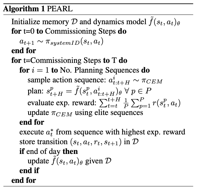
And here’s the pseudocode.
4. Experimental Setup
I’ll now explain the experiments we setup to test the effectiveness of PEARL.
4.1 Environments
Experiments conducted in Energym, an open-source building simulation platform built atop EnergyPlus. We run tests in three buildings:
| Mixed-Use | Offices | Seminar Centre | |
|---|---|---|---|
| Location | Athens, Greece | Athens, Greece | Billund, Denmark |
| Floor Area (m\(^2\)) | 566.38 | 643.73 | 1278.94 |
| Action-space dim | \(\mathbb{R}^{12}\) | \(\mathbb{R}^{14}\) | \(\mathbb{R}^{18}\) |
| State-space dim | \(\mathbb{R}^{37}\) | \(\mathbb{R}^{56}\) | \(\mathbb{R}^{59}\) |
| Thermal Zones | 13 | 25 | 27 |
| Sampling Period | 15 minutes | 15 minutes | 10 minutes |
| Controllable Equipment | Thermostats & AHU Flowrates | Thermostats | Thermostats |
- Standard MDP setup with state-space \(\mathcal{S} \in \mathbb{R}^{d_s}\), action-space \(\mathcal{A} \in \mathbb{R}^{d_a}\), reward function \(r(s_t, a_t)\), and transition dynamics \(p(s_{t+1}|s_t, a_t)\).
- Agent attempts to maximise return \(G_t = \sum_H \gamma^H r(s_{t+H}, a_{t+H})\), where \(\gamma \in [0,1]\) is a discount parameter, and \(H\) is a finite time horizon.
We use an open-source building simulation platform called Energym in which we run experiments in three buildings: a mixed-use (industrial) facility in Athens, Greece, and Office block also in Athens, Greece, and a Seminar Centre in Billund, Denmark. You can see from the table that they vary in physical size, and they vary in the dimensions of their action and state spaces, and number of thermal zones. The state spaces are generally composed of a range of temperature, humidity and pressure sensors, both internal and external. The action spaces are composed of thermostat control in all cases, and in the mixed-use case the flowrates through the Air Handling Units can be controlled continuously.
We follow the standard reinforcement learning setup where we model the environment as a Markov Decision Process (MDP) with a state-space, action-space, and transition function defined as a probability distribution across the next state given a current state and action. We assume full access to the reward function, which I’ll discuss in a second.
4.2 Baselines
We compare the performance of our agent against several strong RL baselines, and an RBC:
- Soft Actor Critic (SAC; (Haarnoja et al., 2018))
- Proximal Policy Optimisation (PPO; (Schulman et al., 2017))
- MPC with Deterministic Neural Networks (MPC-DNN; Nagabandi et al. (2018))
- RBC: a generic controller that modulates temperature setpoints following the simple heuristics
- Oracle (Pre-trained SAC): an SAC agent with hyperparameters optimised for each environment and trained for 10 years prior to test time.
We compare the performance of PEARL with several RL baselines. These include Soft Actor Critic, as its general accepted to be the best performing, lowest variance model-free algorithm; PPO because it’s popular in production and a seminal model-free algorithm; MPC-DNN as a high performing model-based method and the best performing algorithm in the smart-building literature. We use a pre-trained SAC agent as an oracle i.e. we overfit the hyperparameters to each building and train for 10 years in each building prior to deployment. And we use a generic rule-based controller.
4.3 Reward Function
Linear combination of an emissions term and a temperature term:
$$ r[t] = r_E[t] + r_T[t] $$
with:
$$r_{E}[t] = - \phi \left(E[t] C[t] \right)$$
$$ \begin{equation} r_T^i[t]= \begin{cases} 0:& T_{low} \leq T_{obs}^i \leq T_{high} \ -\theta \min [(T_{low} - T_{obs}^i[t])^2, ; (T_{high} - T_{obs}^i)^2]: & \text{otherwise} \ \end{cases} \end{equation} $$
where:
- \(E[t], C[t],\) and \(T_{obs}^i[t]\) are energy-use, grid-carbon intensity and observed temp. at time \(t\).
- \(\theta\) and \(\phi\) are tunable hyperparameters to set relative emphasis of emission minimisation over temp.
- \(\theta\) » \(\phi\)
- \(T_{high}\) and \(T_{low}\) are upper and lower bounds on thermal comfort.
The task is to maximise reward (specifically over time horizon \(H\)) for one year without prior knowledge, historical data or access to the simulator a priori.
The reward function that each agent can access is a linear combination of an emissions term and a temperature term. The emissions term is the product of energy-use and grid carbon intensity at timestep \(t\). The temperature term is 0 when the temperature falls within a zone of thermal comfort with upper and lower bounds, and is penalised quadratically when it falls outside this range. Here, theta and phi are tunable hyperparameters that set the relative emphasis of emissions minimisation to thermal comfort. The task for each agent is to maximise this reward over time horizon H without any prior knowledge, historical data or access to the simulator a priori.
5. Results and Discussion
I’ll now present some results, starting with the emissions and thermal performance of the agents.
5.1 Performance

Here we have performance for the aforementioned three environments over the course of one year. The top row of charts are cumulative emissions and the bottom row represents thermal comfort over the time period. If we start by looking at the top row, the key colours are red (RBC), black-dashed (pre-trained SAC, representing pseudo-optimal performance) and green (PEARL). We find that PEARL minimises emissions in the mixed-use facility, reducing emissions by 31% compared to the RBC. In the Office environment, PEARL outperforms each of the RL agents but is bested by the RBC, and in the seminar centre all controllers perform almost identically.
From a temperature perspective, PEARL outperforms all of the other RL agents, controlling the building safely throughout the year. The green band thermal comfort constraints, and PEARL only misses it once in mixed-use facility, twice in the office and never in the seminar centre. In contrast the other RL algorithms miss it quite regularly. For reference, the brown line represents outdoor temperature which is the main system disturbance.
5.1 Performance
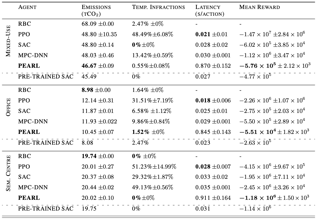
Here’s a table of the results in more detail. We present the mean and standard deviation of three runs of the experiment–bold items are the best performing. In addition to the plots from the previous slide, here we report action latency and mean reward. Though PPO has the lowest action latency, all agents select actions quickly enough that we do not need to worry about compute overhead if we were taking these actions in the real environment. The final column is mean daily reward, we see that PEARL maximises reward in each of the environments i.e. it does the best job of minimising emissions whilst maintaining thermal comfort. I also want to point out the performance of the pre-trained SAC agent; it outperforms all agents in each environment as we’d expect, but not by a huge amount. This suggests that we are not far off the performance ceiling in this setup.
A key, high-level observation from these results is that we have reduced emissions massively in the mixed-use facility, but not in the other two environments. If we go to the table of describing the environments, we see that the only difference between the mixed-use facility and the rest is that the agent has access to AHU flowrate actuation. Indeed, the rest of the setup is not dissimilar to the office otherwise - same weather, similar state-spaces etc. In the other settings where only temperature setpoints are modulated, defining rules that mediate this behaviour is quite straightforward, but designing rules that unpick the complexity of a combination of setpoints and AHU flowrate throughput is more difficult. This result would suggest that RL agents can only significantly improve performance when there’s an added level of complextity beyond thermostat regulation.
5.2 System Identification

Planning loss = \(\sum_{n=1}^{100} MSE(\hat{s}{t:t+H}^n, s{t:t+H}^n)\)
One part of the system that we perform further analysis on is the system identification policy. In these charts, I’m varying the length of the commissioning period to assess how that affects performance over the first month of operation – we only look at the first month because any effect of system identification is subsumed by data collection beyond this point.
We vary the length of system ID in the range 1hr-72hr and then measure the planning loss on a test set of 100 random state-action trajectories obtained from a different controller sampled from other times in the year. The planning loss is the sum of the state prediction MSEs. On the left is the planning loss right at the end of the commissioning period, and on the right is the change in planning loss for the same test set as the agent collects more data from the environment. To be clear, the agent is interacting with the environment, collecting data, and updating its model parameters at the end of each day so as to improve its model.
We find that, as expected, the longer the system identification period, the more accurate the model predictions are at the end of that period. However, we also see that despite this initial discrepency, generally model performance converges after a few days of interaction, suggesting the data collected during system ID becomes quickly subsumed by other data in the environment. There is tradeoff between commissioning complexity and performance at the start of deployment. My conclusion from this analysis is that although we get better performance initially with a longer system ID period, the convergence in performance after a few days means that a shorter commissioning period remains practical.
5.3 Agent Decomposition
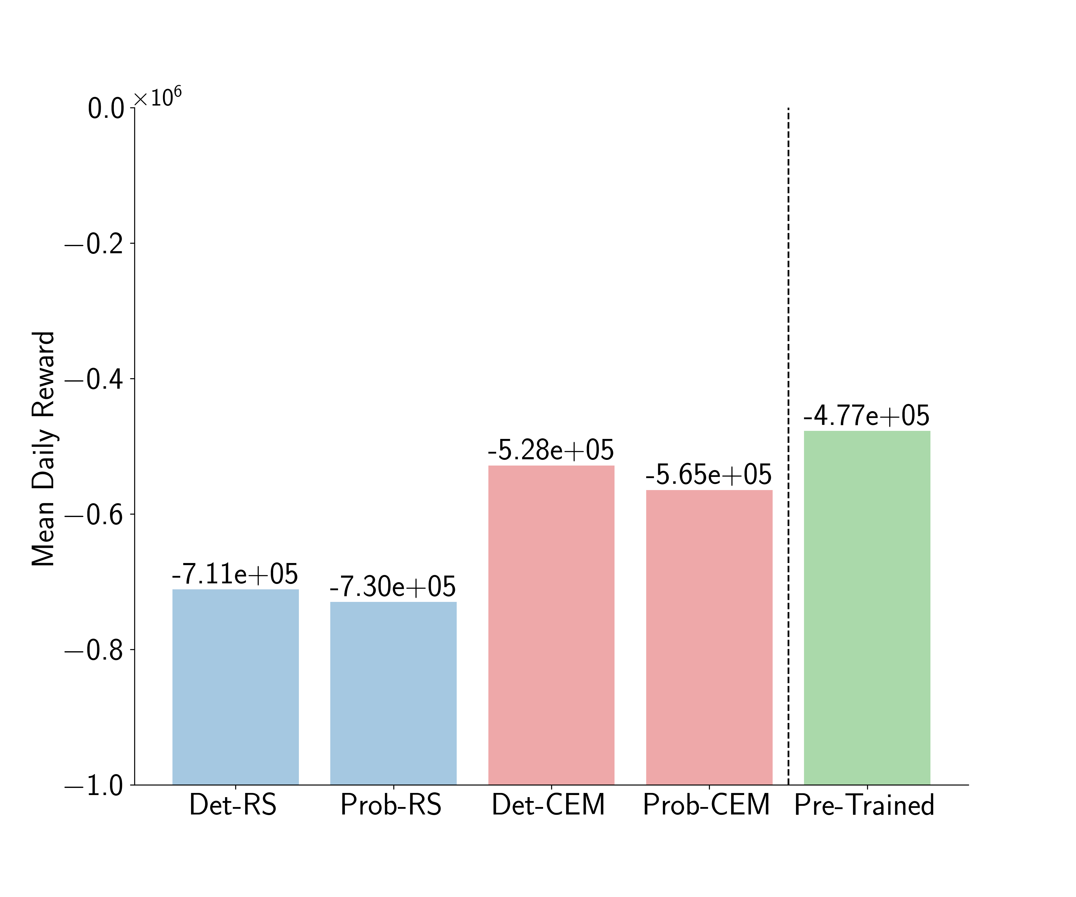
My final chart is a decomposition of the components of PEARL that lead to its success. When compared with MPC-DNN, the other model-based technique used in this study, there are two components that are different: the use of probabilistic rather than deterministic models, and the use of Cross-Entropy Maximisation over Random Shooting as an action-selection mechanism. Here, I plot the mean daily reward of four different instantiations of PEARL with combinations of these two components. In blue, actions selected with random shooting and the dynamics modelled using probabilistic and deterministic ensembles, and in red actions selected with CEM and the dynamics modelled again using probabilistic and deterministic ensembles. In green we report the performance of the pre-trained model for reference. We find that performance correlated more with the choice of optimiser than it does with the choice of network, which is interesting and contrary to other results in the literature. Indeed, other authors have shown empirically that probabilistic ensembles perform better than deterministic ensembles, but that is not what we observe. Generally, they are shown to be better in environments that are complex, and this perhaps suggests that the problem is not complex enough to fully utilise probabilistic models.
6. Limitations, Future Work and Conclusions
I’ll finish with a discussion of some limitations and future work.
6.1 Limitations
- Sensor coverage:
- Energym simulations provide large state-spaces; unclear how performance would be affected by lower sensor coverage.
- We assume temporally consistent sensor readings, sensor dropout is likely in the real-world which violates MDP.
- Action-space complexity:
- How complex is too complex?
- How often can we control AHU flowrate in the real world?
- Environments:
- Cannot draw concrete conclusions from tests in three environments for 1 year.
I see three key limitations with this work. Firstly sensor coverage: energym provides large state-spaces with lots of sensors, in this work I have investigated how performance would change with less sensors. I also assume that the agent receives temporally consistent sensor readings, but sensor dropout is likely in the real world which violates the MDP.
Second, I suggested that action-space complexity correlates with agent performance, but how complex is too complex? It’s unclear at the moment at what point control may breakdown or become unsafe. Further, how likely are we to be able to control AHU flowrate in the real world?
Third and finally, this analysis is limited by the functionality of Energym, which only provides three useful environments. It’s hard to draw concrete conclusions from three environments and of course we’d like to test generality across further environments.
6.2 Future Work
- Test in-situ.
- Non-stationarity: how do we deal with it rigorously?
- Scale-up simulations: can we generate two/three orders of magnitude more building sims? We could draw EnergyPlus input files from some representative distribution of building types and train one agent across them.
- Sensor dropout: can we mitigate inconsistent readings with Latent ODEs?
6.3 Conclusions
- Efficiently controlling heating and cooling systems in buildings is a useful climate change mitigation tool.
- To scale RL control to every building in the world, we must bypass expensive-to-obtain simulators.
- We show that it is possible to control heating and cooling systems safely and by combining system ID and model-based RL.
- Efficiency delta appears to correlate with action-space complexity.
- Choice of action-selection optimizer appears key to safe control.
Thanks!
Website: https://enjeeneer.io
Slides: https://enjeeneer.io/talks/
Twitter: @enjeeneer
Questions?
7. References
Chua, K., Calandra, R., McAllister, R., and Levine, S. Deep reinforcement learning in a handful of trials us- ing probabilistic dynamics models. arXiv preprint arXiv:1805.12114, 2018.
Cullen, J. and Allwood, J. The efficient use of energy: Tracing the global flow of energy from fuel to service. Energy Policy, 38(1):75–81, 2010
Ding, X., Du, W., and Cerpa, A. E. Mb2c: Model-based deep reinforcement learning for multi-zone building con- trol. In Proceedings of the 7th ACM International Con- ference on Systems for Energy-Efficient Buildings, Cities, and Transportation, pp. 50–59, 2020.
Haarnoja, T., Zhou, A., Abbeel, P., and Levine, S. Soft actor- critic: Off-policy maximum entropy deep reinforcement learning with a stochastic actor, 2018. URL https: arxiv.org/abs/1801.01290.
Lakshminarayanan, B., Pritzel, A., and Blundell, C. Simple and scalable predictive uncertainty estimation using deep ensembles. Advances in neural information processing systems, 30, 2017.
Lazic, N., Lu, T., Boutilier, C., Ryu, M., Wong, E.J., Roy, B., Imwalle, G.: Data center cooling usingmodel-predictive control. In: Proceedings of the Thirty-second Conference on Neural InformationProcessing Systems (NeurIPS-18). pp. 3818–3827. Montreal, QC (2018)
Nagabandi, A., Kahn, G., Fearing, R. S., and Levine, S. Neural network dynamics for model-based deep reinforce- ment learning with model-free fine-tuning. In 2018 IEEE International Conference on Robotics and Automation (ICRA), pp. 7559–7566. IEEE, 2018
Scharnhorst, P., Schubnel, B., Fern ́andez Bandera, C., Sa- lom, J., Taddeo, P., Boegli, M., Gorecki, T., Stauffer, Y., Peppas, A., and Politi, C. Energym: A building model library for controller benchmarking. Applied Sciences, 11 (8):3518, 2021
Schulman, J., Wolski, F., Dhariwal, P., Radford, A., and Klimov, O. Proximal policy optimization algorithms. arXiv preprint arXiv:1707.06347, 2017.
Valladares, W., Galindo, M., Guti ́errez, J., Wu, W.-C., Liao, K.-K., Liao, J.-C., Lu, K.-C., and Wang, C.-C. Energy optimization associated with thermal comfort and indoor air control via a deep reinforcement learning algorithm. Building and Environment, 155:105 – 117, 2019. ISSN 0360-1323
Wei, T., Wang, Y., Zhu, Q.: Deep reinforcement learning for building hvac control. In: Proceedings of the 54th Annual Design Automation Conference 2017. DAC ’17, Association for ComputingMachinery, New York, NY, USA (2017).
Zhang, C., Kuppannagari, S. R., Kannan, R., and Prasanna, V. K. Building hvac scheduling using reinforcement learning via neural network based model approximation. In Proceedings of the 6th ACM international conference on systems for energy-efficient buildings, cities, and trans- portation, pp. 287–296, 2019a.
Zhang, Z., Chong, A., Pan, Y., Zhang, C., and Lam, K. P. Whole building energy model for hvac optimal control: A practical framework based on deep reinforcement learn- ing. Energy and Buildings, 199:472–490, 2019b.